Guide
The Powersim Sun simulation leads you through a series of steps in which you both provide input on various parameters and see results.
Throughout the user interface, a light orange color is used to denote that a table cell is editable. Non-colored cells are output only.
Also, remember that the various graphs of the user interface can be rescaled at any time by using the
![]() Autoscale now command, or by pressing the F9 shortcut key.
Autoscale now command, or by pressing the F9 shortcut key.
Start page

The Start page gives an overview of the main steps of the Powersim Sun simulation.
You can start an analysis in two different ways. Use the Start new analysis button to start a completely new analysis and let configuration data (info about solar panels, inverters, electricity consumption, etc.) be read from Excel. A dialog will briefly appear while configuration data is read from Excel. Use the Rerun current analysis button to start an analysis without loading data from Excel. In this case, the data loaded the previous time you ran an analysis will be used. This option is for example useful if you have started an analysis by double-clicking a game file (.sig file) containing a previous analysis. The configuration data in Excel may have changed and you probably don't want these changes to affect the existing analysis.
Energy Consumption

On the Energy Consumption page, you provide information about the expected consumption of electric energy over the course of a year, and you determine various parameters related to electricity prices. From here you can also decide whether to make prices subject to a set of policies that control how the prices vary over years.
Energy consumption
The electric energy consumption is given as monthly values for a whole year. In calculations involving multiple years, the monthly pattern is repeated for each year. The upper graph depicts the monthly values as hourly averages (in kWh/h) over the year. The graph is read only on this page, so push the Modify button to go to the page where you can edit the values that the graph is based on.
Energy usage & costs
This section just lists the consumption of electric energy for a whole year and its associated costs.
Electricity prices
The main component of the electricity price is the spot price, which is read as hourly values from Excel (see configuration). The hourly spot price is typically taken from the most recent historical data and is used for the initial (basis) year of the simulation. The price policy (if included) for the spot price determines how the price varies for subsequent years.
On top of the fluctuating spot price, a flat spot price premiums and a flat grid rent are added. You enter the values (in currency per kWh) for these two in the light-orange-colored cells. Also premiums and rent can be subject to a price policy if you desire. Push the Define price policy button to determine policy details.
Energy Consumption – Details
On the Energy Consumption – Details page you can specify your yearly consumption of electric energy in detail. You provide 12 monthly consumption values, one for each month as well as a daily pattern.
Data resolution
The monthly consumption is combined with a daily usage pattern to produce an hourly usage for a whole year as depicted in the uppermost read-only graph.
Monthly data
The monthly data is given as 12 values measured in MWh. You can set these values by dragging the graph in the middle of the page or by entering values in the table to the right.
Daily pattern
The 24 (one for each hour) values of the daily pattern is overlaid the monthly data to produce the overall hourly consumption graph for a year. You can choose between four different predefined patterns, but note that these are just starting points. Select the pattern that is closest to your expected daily consumption variation and then drag the curve to the desired shape. The unit of measurement is percent but the absolute number for each hour is not important per se; it is the relative difference between the percent numbers that matters. In the end, each number is divided by the overall sum to give a proper percentage of the daily consumption for that given hour.
Energy Consumption – Purchase price policy
On the Energy Consumption – Purchase price policy page you determine how various price elements of the simulation vary after the initial year. The policy applies to price elements for buying electricity from the grid and plays an important role in the return on investment calculations, influencing the estimated time until the investment in renewable energy has paid itself.
Purchase price policy
The spot price is read from Excel as hourly values over a period of a year. A spot price premiums and a grid rent are added on top of the spot price, and you can edit these two fixed prices in the light-orange-colored cells. The year average of the spot price and the two fixed values constitute the basis for the price policies.
Policy for each price element
Here, you can select a policy for all three of the elements involved in the electricity purchase price: the spot price, the spot price premiums, and the grid rent. Only one is shown in the graph at a time; select which one in the dropdown above the graph.
If you check the Manual edit of price elements box, the graph curve that shows how the selected element varies after the initial year is editable. Select the curve and drag one of the handles that appear on the curve. Note that you can swipe to adjust the curve to the desired profile. Alternatively, you can uncheck Manual edit of price elements and then use the slider to the right to set a yearly growth in percent. Note that the check box setting applies to all price elements; you cannot select manual editing on an individual element basis.
In any case, the value for the current (initial) year cannot be changed; the policy is about subsequent years. For the spot price premiums and the grid rent, the first value is set to the fixed value you have entered. For the spot price, which is given as hourly values for the initial year, the initial year's average is used as the first (unchangeable) value.
Location & Solar Panels

On the Location & Solar Panels page, you give the location of the building for which you plan a solar panel installation, and you provide important information about how the solar panels will be positioned.
Note that in this version of Powersim Sun, the solar panels are assumed to be mounted on a surface of the building.
Location
You give the location with the help of Google Maps. Push the Find location... button, and a dialog with a map appears. If you know the address of the location, enter it in the edit field at the top and then push the Search button. The map will scroll to the entered location. If you don't have the exact address you can scroll and zoom in the map until you see the target location and then just click in the map.
In either case, when the red map indicator points to the desired location, push Ok to use it in the simulation. The dialog is closed and you will see that the location's latitude and longitude (as well as its address) are shown on the Location & Solar Panels page.
Note that you can use all of the powerful facilities of Google Maps inside the dialog, such as for example switch between map or satellite views. The dialog is sizable so you can make the map larger than its default size.
Solar panel facing direction and tilt angles
Determine how you plan to position the panels by entering a facing direction angle and a tilt angle.
The facing direction angle is often also referred to as the azimuth angle and is in Powersim Sun measured clockwise from a south base line. The tilt angle reflects at what angle from horizontal the panels are to be tilted, ranging from 0 degrees (flat roof) to 90 degrees (wall mount).
If you want to fine-tune the positioning please push the Panel details button.
Location & Solar Panels – Panel details
If your building prospect gives you freedom with respect to choosing panel facing direction and/or tilt angles, you can fine-tune the positioning of the solar panels on this page with the help of a chart that shows solar energy utilization for any day of the year.
Fine-tune panel position
In the graph, the green filled area shows the utilization of solar energy together with the solar elevation angle. The larger the area, the better is the utilization. Select any day of the year for which to check and change panel facing direction and/or tilt angle by dragging the red needles in the gauges to the right. Alternatively, you can enter the angles in the light-orange-colored cells below each of the gauges.
Tilt angle details
You can get further assistance with determining the tilt angle on the page that appears if you click the green-colored Tilt Angle Details button.
Location & Solar Panels – Tilt angle details
On this page you can further fine-tune the solar panel tilt angle, and you get help to do so through a graph that shows solar energy utilization for a given time of day throughout a whole year. The time of day is preset to the point of the day that gives the highest exposure on the panel based on the panel facing direction. The facing direction (azimuth angle) cannot be changed on this page; it is shown in a read-only gauge.
The green-colored, filled area in the graph depicts the solar energy utilization (the larger the area, the better is the utilization). The gauge in the lower left corner also shows this utilization factor. The higher the indicator is, the better the utilization is. Change the tilt angle by dragging the red needle of the tilt angle gauge or by entering a number in the corresponding light-orange-colored cell and then observe the effect on the utilization.
You can also change the time of the day from the preset value to see how the tilt angle influences on times of the day that are not optimal with respect to exposure. The time of the day is changed by adjusting the slider to the right of the clock.
Location & Solar Panels – Investments
When you enter this page, energy production is calculated based on specified location, panel facing direction and panel tilt angle. When the "Calculating. Please wait ..." message has disappeared you are ready to specify the type and number of solar panels you want to use. In addition, you need to specify which inverter type to use for your solar panel installation, and give an estimate of the overall installation cost of the facility.
Solar panels
In the dropdown list, select which of the available solar panels you want to use. The list is generated from the Solar Panels Worksheet in the Excel configuration file.
Furthermore, you need to specify how many of the selected solar panels you want. Use the slider or write the number in the light-orange-colored cell. Based on the panel's characteristics the resulting solar panel area (in square meters) is calculated for you.
Note that calculations are done for all combinations of panel types in parallel, making it very quick to switch panel type — also on later pages.
Inverters
In the dropdown list, select which of the available inverters you want to use. The list is generated from the Inverters Worksheet in the Excel configuration file.
The number of inverters needed for the selected inverter type and panel type is calculated for you based on the listed array to inverter ratio from the inverter data in the Excel configuration file. This ratio is an array of solar panels' power rating (n * Pmax) divided by the inverter's size (power rating). You can adjust the number of inverters up and down by using the slider just below the number box. The resulting array to inverter ratio is shown alongside the listed ratio.
Peak production
Given the selected solar panel type and the number of panels, see the expected peak production. This value is the panel producer's reported peak value times the number of panels selected, and gives a theoretical maximum effect for your facility.
Monthly energy production
The graph and the accompanying table at the bottom shows the resulting monthly energy production (measured in kWh) based on the building prospect's location as well as selected solar panels and inverters. In the table you can also see the production for a whole year.
Investment costs
Under this section there is just one input value; you need to provide an estimate of the overall installation cost for the facility in the light-orange-colored cell. Note that the installation costs also include costs relating to installation of battery packs, if applicable. You specify whether to include battery packs on the next wizard page. Solar panel costs and inverter costs are calculated for you and added to the installation cost to give a total investment cost that is used in subsequent economic calculations.
Location & Solar Panels – Error
If an unexpected error happens during calculation of solar energy production (using Meteonorm™), you will be led to this page. The detailed description on the page provides information about what went wrong and what you can do to correct the error.
Battery Packs

On the Battery Packs page you decide whether to include batteries to store (for later use) produced solar energy when energy consumption is low. Select one of the available battery types from the dropdown list and then specify how many batteries of this type to use. If battery technology is not a viable option for your facility, set the number of batteries to zero and continue to the next page.
Battery packs
In the dropdown list, select which of the available battery types you want to use. The list is generated from the Batteries Worksheet in the Excel configuration file.
Furthermore, you need to specify how many of the selected batteries you want. Use the slider or write the number in the light-orange-colored cell.
Investment costs
Based on the selected battery type's list price (one of the properties read from the Excel input file), investment cost for batteries is calculated for you. This cost is shown together with the overall investment cost.
Production & consumption
The graph shows the consumption and production of energy in your installation for a selected day of the year. Even if you have decided to not have any battery packs in the installation this graph can be useful to inspect produced solar panel energy vs. consumption for a selected day.
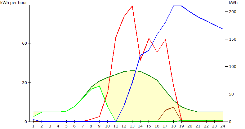
The graph has two sets of curves. Four curves show production/consumption measured in kWh per hour. These values can be read on the left axis. The two blue curves are battery levels measured in kWh, and the values can be read on the right axis.
If you change the number of battery units or change the selected day of the year, you may need to press F9 on the keyboard to rescale the graph. Note that the two blue curves (on the right axis) are scaled independently of the other curves.
 |
The dark green curve shows the total energy consumption for the facility through the selected day. The energy values are per hour and can be read on the left axis. |
 |
The light green curve shows the consumed energy that is bought from the grid. The energy values are per hour and can be read on the left axis. |
 |
The yellow area between the green consumption curves illustrates the amount of solar energy consumed that day. |
 |
The dark blue curve shows the energy that is stored in the battery. This is accumulated energy that can be read on the right axis. |
 |
The light blue curve is a constant value that shows the total battery capacity. The batteries are fully charged when the dark blue curve reaches this line. |
 |
When the battery is fully charged you may sell excess energy to the grid. This is displayed with the brown curve, and its values can be read on the left axis. |
Return on Investment

On the Return on Investment page, you see the effects of your planned investment in solar panel technology and battery packs through a full year of use. The other key element on this page is the estimated time until the investment has paid itself.
Sell to grid
Use the check button to decide whether excess solar energy is sold to the grid or not (if your energy company gives you this opportunity). Push the Define price policy button to determine sales price policy details. The average sales price used for economic calculations is also listed here (will be zero if you choose not to sell to grid).
Investments
You can still make changes to your decisions regarding investments in solar panel technology and battery packs, while seeing the effect over the course of a year. The input controls are the same as on the previous pages.
Costs, sales and savings
Here the total investment costs is listed alongside sales to grid and savings per year. Savings is former electricity costs less new electricity costs plus sales to grid, giving you a measure on how much the investment in new technology saves you per year.
ROI for your installation
Here the number of years and months it takes before the investment has paid itself is shown alongside a graph that depicts the development of the net present value of the investment for the first 25 years.
Production & consumption
The graph displays the same curves as on the previous page (see explanation for legend), but now for the entire initial year of the simulation. You can select three different resolutions of the graph: Day, week, and month.
Return on Investment – Sales price policy

On the Return on Investment – Sales price policy page you determine how the electricity sales price policy varies after the initial year. The policy applies to selling electricity to the grid and plays an important role in the return on investment calculations, influencing the estimated time until the investment in renewable energy has paid itself.
Sales price
Here you can select whether to base the policy on a fixed price or on the purchase spot price. In the first case, you just enter the fixed price in the corresponding light-orange-colored cell. In the second case, you can enter the fixed premiums that is added to the fluctuating purchase spot price.
Policy for sales price
If you check the Manual edit of sales price box, the graph curve that shows how the sales price varies after the initial year is editable. Select the curve and drag one of the handles that appear on the curve. Note that you can swipe to adjust the curve to the desired profile. Alternatively, you can uncheck Manual edit of sales price and then use tOn he slider to the right to set a yearly growth in percent.
In any case, the value for the current (initial) year cannot be changed; the policy is about subsequent years. For the fixed price alternative, the first value is set to the fixed value you have entered. For the spot price with premiums alternative, where the purchase spot is given as hourly values for the initial year, the initial year's average spot price plus the entered premiums is used as the first (unchangeable) value.
Summary

The Summary page presents an overview of the main parameters of the current analysis with special focus on the return of investment for the installation. Note that you can still make last-minute changes to some of the parameters, and observe the effect on the return on investment.
Summary information
If you do analyses for multiple prospects or if you are working with multiple alternatives for a single prospect, it is a good idea to save the analysis for later use. If you push the Save... button, you are allowed to save the current analysis as a so-called game file (extension .sig). You can give this file any name you want.
When you later double-click such a file in Windows Explorer, the analysis will be re-opened in Powersim Studio with the summary page active and showing the exact same parameters as at save time. You can then use the Back button to go back to any of the pages to view results or even make changes. Note that if you go all the way back to the start page, you would normally choose the Re-run current analysis button to go through the steps of the wizard again. With this option, no configuration data (which might have changed since the game file was saved) will be read from Excel, and you are sure that you are working with the exact same data as previously. On the other hand, if you want to apply changes in the configuration data (solar panel characteristics, inverter characteristics, etc.) to the previous analysis, you should of course select the Start new analysis button, but please be aware that also consumption data is read from Excel, possibly overwriting changes you did in the Powersim Sun user interface in this regard before saving the game file.
The installation
Here you find the address of the analyzed installation as well as selected panel positioning information.
Investments
Here you find a summary of your investments in solar panels, inverters and battery packs.
Consumption & production
See total yearly energy consumption vs. energy production.
Costs, sales & savings
This section shows the electricity costs before and after investment in solar energy technology together with sales to grid. Savings is former electricity costs less new electricity costs plus sales to grid.
Investment costs
This section gives the total investment costs together with the costs for its three components: solar panels, inverters and battery packs.
Return on investment
The return on investment calculation repeats the initial year's development for subsequent years, but takes price policies into account. This involves net present value (NPV) calculations making use of a discount rate that you are free to change.
The number of years and months it takes for the investment to pay itself is shown in the lower left corner. The same information can be read from the graph, which shows the net present value of the investment for the 25 first years. When the NPV value goes positive, the investment has paid itself. Note that the graphs shows only 25 years, no matter how long it takes before the investment pays itself.